I am a huge fan of Excel Power Query! You can automate, clean and transform your data, compare tables and so much more. In this post I show you how to append tables within an Excel workbook.
Append tables within an Excel workbook
When you need to append tables from the current workbook, don’t start it manually with copy-paste. Excel Power Query is here to help!
Power Query is one of my favorite tools in Excel. Let’s see how to use it in this case.
You can download the sample file here:
I have 3 worksheets with one table on each.

I need one table that contains all the rows from these separate tables.
To solve this with Power Query, first, you have to name the tables correctly.
It is important to differentiate the tables you want to append from the result table that the query gives you at the end. It can be a word in every table’s name, for example, January_data, Feburary_data, etc. and you skip data tag from the result table.
Or in reverse, you name the result table as Total or Year_total, and Total should not be in the names of the tables. It is needed for the filtering step in the query. Without this, the query keeps adding the result table with every single refresh and you’ll get a table with wrong data.
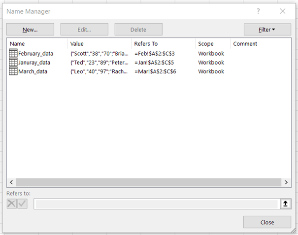
I named the tables in the sample file January_data, February_data, and March_data

Now that it is done, let’s create a blank query!
Append tables – Create a blank query
To do so, navigate to Data tab, Get data -> From other sources -> Blank query

The query editor opens. In the formula bar type this M function:
=Excel.CurrentWorkbook()
If you have newer version, Excel will show you the list so you can choose this function. The coding is case sensitive so you have to type it as shown (if you can’t choose).

Press Enter, then you will see the list of the tables in the workbook.

Append tables – Filter tables
I know what the problem will be if we do not filter, so instead of getting back here at the end, I show you the step that has to be included.
In Name column click on filter button -In Name column click on filter button – Text Filters -> Ends With…

Type data or _data. It is case-sensitive, so if you use capitals, write the words accordingly. Then click OK.

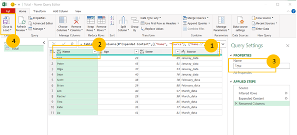
Choose which columns you want to see in the result table, I choose all of them, then uncheck the Use original column name as prefix. Then OK.

In this step, you can clean your data, remove columns, add new columns, adjust data types, etc.
I just renamed the last column to Source and the first column to Name. Then renamed the query as Total. This will be the table name automatically.


Load it to Excel, choose Close & Load from the Home tab.
The result table is on a new worksheet named Total. 11 rows are loaded.

It seems OK. Let’s add a new table, refresh it and see if it is working correctly
Append tables – Refresh the query
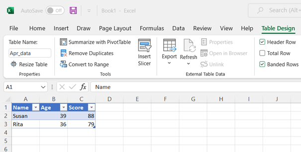
Add a new worksheet and type some data. Create a table from it and name it following the rules above: Apr_data. (or April_data)

Go back to the Total worksheet to see what will happen. Press Alt+F5 to refresh (or Data tab -> Refresh, or right-click on the table -> Refresh. There are multiple ways to choose and to confuse 😊 )
It is working, plus 2 rows added from the April table.

I hope you enjoyed my tip! Use it in your files and keep practicing.
Don’t forget to connect me via LinkedIn. 😊
More posts in English
You can find more posts in English under this category
